#3 Spreadsheet Basic Formatting

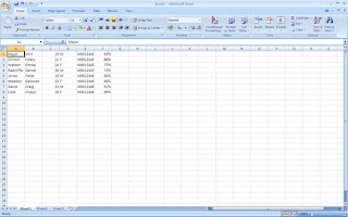
Once raw data is entered onto the worksheet, we need to apply various formatting to make the worksheet look more attractive and also to be able to interpret what the data is trying to show. Take a look at the worksheet below:

Use this link to download the workbook in the image above to try the exercise below.
(Click file > Download as > Excel)

As you can see some data has been entered on the worksheet. Active cell has a reference of A1. However without any headings or formatting one cannot tell what the data represents. Try carrying out the following instructions:

1. Insert an entire row: Select the home tab, go to group named cells and select the command button labelled Insert with a little arrow. Now click Insert sheet Rows.
   
   
2. Enter the following:
   In cell reference A1 write: Surname
   In cell reference B1 write: First Name
   In cell reference C1 write: Age
   In cell reference D1 write: Gender
   In cell reference E1 write: Student ID
   In cell reference F1 write: Attendance
3. Select cell reference A1 hold the right button on the mouse down and drag cursor from A1 to F1 to select all cells from A1 to F1.
4. Making the selected cell range bold: Select the home tab, go to group named font and select the command button labelled with a bold B.
5. Formatting row size using AutoFit: Select the home tab, go to group named cells and select the command button labelled Format with a little arrow. Now click AutoFit Column Width.
6. Select cell range from A1 to F9.